One Hot Encoding in Machine Learning: Bridging the Gap Between Categories and Code
Hey there, fellow data enthusiasts! I spend a lot of time thinking about how we prepare data before feeding it to our machine learning models. It’s not the most glamorous part of the job, but it’s arguably one of the most critical. You see, machine learning algorithms, for the most part, speak the language of numbers. They understand vectors, matrices, and numerical values. But what happens when your dataset includes information like “City,” “Product Category,” or “User Role”? These aren’t numbers; they’re categories, labels, or nominal values.
This is where the magic of One Hot Encoding comes into play. It’s a fundamental technique in the data preprocessing toolbox, essential for transforming that seemingly incompatible categorical data into a format that ML models can not only digest but also learn effectively from. If you’re just starting your journey in machine learning, understanding this concept is non-negotiable. Let’s dive in!
What is One Hot Encoding?
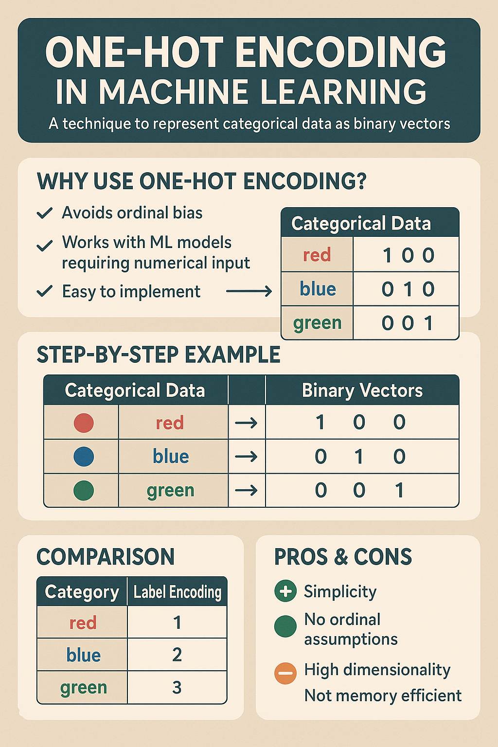
At its core, One Hot Encoding (often abbreviated as OHE) is a process that converts categorical variables into a numerical format suitable for machine learning algorithms. Specifically, it transforms a single categorical column with multiple unique values into multiple binary columns.
Think of it this way: instead of having one column listing different colors like “Red,” “Blue,” “Green,” you’ll end up with separate columns named “Color_Red,” “Color_Blue,” and “Color_Green.” For each row, one of these new columns will have a value of 1 (indicating the presence of that color), while all the others will have 0.
Why is this important? Because many machine learning algorithms (especially linear models like Linear Regression, Logistic Regression, and SVMs, but also useful for tree-based models and others) cannot directly process text labels or categorical integers if those integers imply a false sense of order or magnitude.
Real-World Applications
You’ll find OHE applied in countless scenarios:
- E-commerce: Encoding ‘Product Category’ (Electronics, Apparel, Books) or ‘Brand’.
- Healthcare: Encoding ‘Medical Condition’ or ‘Treatment Type’.
- Finance: Encoding ‘Loan Type’ or ‘Customer Segment’.
- Housing Data: Encoding ‘Neighborhood’, ‘Property Type’ (House, Condo, Townhouse), or ‘Number of Bedrooms’.
- Natural Language Processing (NLP): Encoding words or tokens (though often superseded by embeddings for large vocabularies).
How Does One Hot Encoding Work? An In-Depth Look
Youtube Channel :Mısra Turp
Let’s break down the process step-by-step. Imagine you have a dataset about fruits, and one of the columns is ‘Flavor’. The unique flavors are ‘Sweet’, ‘Tart’, and ‘Bitter’.
Original Data:
| Fruit | Flavor |
|---|---|
| Apple | Sweet |
| Lemon | Tart |
| Grape | Sweet |
| Bitter Melon | Bitter |
The Encoding Process:
- Identify the Categorical Column: We target the ‘Flavor’ column.
- Find Unique Categories: List all unique values: ‘Sweet’, ‘Tart’, ‘Bitter’.
- Create New Binary Columns: For each unique category, create a new column. We’ll have ‘Flavor_Sweet’, ‘Flavor_Tart’, and ‘Flavor_Bitter’.
- Assign Binary Values: For each row in the original data, go to the new columns. Place a
1in the column corresponding to the row’s original category and0in all other new columns for that row.
Encoded Data:
| Fruit | Flavor_Sweet | Flavor_Tart | Flavor_Bitter |
|---|---|---|---|
| Apple | 1 | 0 | 0 |
| Lemon | 0 | 1 | 0 |
| Grape | 1 | 0 | 0 |
| Bitter Melon | 0 | 0 | 1 |
Notice how the original ‘Flavor’ column can now be dropped (or sometimes kept, though typically dropped to avoid perfect multicollinearity if not handled correctly by the algorithm). Each row is now represented numerically based on its category.
Analogy: Checkboxes on a Form
Imagine you’re filling out a survey asking about your preferred ice cream flavors. Instead of writing down the flavor, you check boxes:
- Which flavors do you like? [ ] Chocolate [ ] Vanilla [ ] Strawberry
If you like Chocolate and Strawberry, you’d check those two boxes. OHE is similar for a single category choice. If the survey was “Choose your favorite flavor:”, you’d only check one box. If your favorite is Vanilla, your response could be represented numerically like this:
- Is_Chocolate: 0
- Is_Vanilla: 1
- Is_Strawberry: 0
Each ‘checkbox’ becomes a binary feature, and only the one corresponding to your choice is marked ‘1’.
Mathematical View (Dummy Variables)
Mathematically, One Hot Encoding creates a set of “dummy variables.” For a categorical feature with k unique categories, OHE typically creates k new binary features (though sometimes k-1 is used to avoid multicollinearity, which is a topic for another time, known as the “dummy variable trap”). Each new feature X_i is an indicator function:
\( X_i = \begin{cases} 1 & \text{if the instance belongs to category } i \\ 0 & \text{otherwise} \end{cases} \)
This ensures that each category is represented as a distinct, orthogonal vector in the feature space (e.g., [1, 0, 0], [0, 1, 0], [0, 0, 1]), removing any implied numerical relationship between categories.
Advantages of One Hot Encoding
So, why go through this process? OHE offers significant benefits:
1. Eliminates Misinterpretation of Ordinality
Many machine learning algorithms (like linear models) would interpret integer labels (e.g., encoding ‘Red’ as 0, ‘Green’ as 1, ‘Blue’ as 2) as having a quantitative or ordinal relationship (i.e., 2 is “greater than” 1). For categories without any natural order, this is fundamentally wrong and can lead the model to make incorrect assumptions and learn spurious relationships.
- Practical Scenario: Predicting customer satisfaction based on the ‘Device Used’ category (Mobile, Tablet, Desktop). If you Label Encode these as 0, 1, 2, a linear model might incorrectly assume that using a Desktop (2) contributes “more” to satisfaction than using a Mobile (0), simply because 2 > 0, when there’s no inherent numerical scale to these categories. OHE ([1,0,0] for Mobile, [0,1,0] for Tablet, [0,0,1] for Desktop) prevents this by treating each device type as a separate, unrelated entity.
2. Compatibility with a Wide Range of Algorithms
As mentioned, many algorithms require numerical input. OHE provides a standard way to convert categorical data into a numerical format that is widely accepted. While some tree-based models can handle integer-encoded categorical features directly, OHE is often a safer and more general approach that works across the board.
- Practical Scenario: Building a recommendation system using user features including ‘Country’. One Hot Encoding ‘Country’ allows you to use algorithms like K-Nearest Neighbors (KNN) or Support Vector Machines (SVMs) that rely on distance calculations in a numerical feature space. Simply assigning an arbitrary integer ID to each country would make distance calculations meaningless.
3. Simplicity and Interpretability of Features
The resulting binary features are very straightforward. A value of 1 in a column like ‘Country_USA’ clearly indicates that the data point is associated with the USA. This makes the features easy to understand and interpret, which in turn can help in understanding the model’s decisions (especially with interpretable models like linear regression or logistic regression).
- Practical Scenario: After training a Logistic Regression model to predict whether a user will click on an ad, you examine the model’s coefficients. If the coefficient for ‘City_New York’ is significantly positive, it’s immediately clear that users from New York are more likely to click, assuming all other features are equal. This clear interpretation is possible because OHE created a distinct, unambiguous feature for New York.
Disadvantages and Limitations
While powerful, OHE isn’t a silver bullet. It comes with its own set of challenges:
1. The Curse of High Cardinality
This is arguably the biggest drawback. If a categorical feature has a very large number of unique values (high cardinality), OHE will create a new column for *each* unique value. This can drastically increase the number of features in your dataset.
- Practical Scenario & Problem: Encoding a ‘User ID’ column (if you mistakenly treat it as a categorical feature) or a ‘Zip Code’ feature in a large dataset covering many regions. A dataset with millions of users or thousands of zip codes could result in a huge number of new columns, potentially exceeding the original number of rows! This leads to the “curse of dimensionality,” making training slower, requiring more memory, and potentially causing models to perform poorly due to the sparsity and increased complexity.
- Mitigation: For very high cardinality features, OHE is often not the best choice. Alternatives include:
- Combining rare categories into a single ‘Other’ category.
- Using Target Encoding (Mean Encoding), which replaces categories with the mean of the target variable for that category.
- Applying Feature Hashing, which maps categories to a fixed, smaller number of dimensions using hash functions (though this can introduce collisions).
- Using techniques like Embeddings, particularly common in deep learning, which learn dense, lower-dimensional representations of categories.
2. Creation of Sparse Data
When you create many new binary columns, most of the values in those columns will be 0. The resulting dataset matrix will contain a high proportion of zeros, making it “sparse.”
- Practical Scenario & Problem: In the ‘Zip Code’ example, for any given user, only *one* of the thousands of ‘Zip Code’ columns will have a
1; all others will be0. Handling and processing large, sparse matrices can be computationally inefficient and increase memory usage compared to dense matrices. Some algorithms perform worse on sparse data, while others (like linear models, tree-based models, or specific sparse matrix implementations in libraries) handle it reasonably well. - Mitigation: Use data structures optimized for sparse data (e.g., SciPy’s sparse matrices) when working with libraries like scikit-learn. Choose algorithms known to handle sparsity efficiently. Consider dimensionality reduction techniques if the resulting feature space is too large.
3. Potential for Multicollinearity
Creating a binary column for every category can sometimes lead to perfect multicollinearity, where one new feature can be perfectly predicted from the others (e.g., if you have ‘Male’ and ‘Female’ columns, knowing one is 0 tells you the other must be 1, assuming no missing values). While many ML libraries and algorithms can handle this gracefully, it can sometimes cause issues or make model interpretation less clear, particularly in classical statistical regression.
- Practical Scenario & Problem: Encoding a ‘Gender’ column with categories ‘Male’ and ‘Female’ results in ‘Gender_Male’ and ‘Gender_Female’ columns. If you know ‘Gender_Male’ is 0, you know ‘Gender_Female’ is 1. This perfect dependency is multicollinearity.
- Mitigation: Often, you drop one of the resulting binary columns (creating k-1 columns instead of k). Libraries like Pandas’
get_dummieshave an option (drop_first=True) to do this automatically. However, dropping a column can sometimes slightly reduce interpretability depending on the use case and algorithm.
Putting It Into Practice: A Python Example
Let’s see how to perform One Hot Encoding using Python’s powerful libraries, Pandas and Scikit-learn.
import pandas as pd
from sklearn.preprocessing import OneHotEncoder
from sklearn.compose import ColumnTransformer
from sklearn.pipeline import Pipeline
import numpy as np
# 1. Create a simple DataFrame
data = {'Fruit': ['Apple', 'Banana', 'Orange', 'Apple', 'Grape'],
        'Color': ['Red', 'Yellow', 'Orange', 'Red', 'Green'],
        'Taste': ['Sweet', 'Sweet', 'Sweet', 'Sweet', 'Sweet'],
        'Price': [1.0, 0.5, 0.75, 1.1, 2.0]} # Add a numerical column
df = pd.DataFrame(data)
print("Original DataFrame:")
print(df)
print("-" * 30)
# 2. Using Pandas: pd.get_dummies()
# This is often the simplest method for basic dataframes outside of pipelines
df_encoded_pandas = pd.get_dummies(df, columns=['Color', 'Taste'], drop_first=False)
print("DataFrame after One Hot Encoding (using Pandas get_dummies):")
print(df_encoded_pandas)
print("-" * 30)
# Using drop_first=True to avoid multicollinearity (optional but common)
# df_encoded_pandas_dropped = pd.get_dummies(df, columns=['Color', 'Taste'], drop_first=True)
# print("\nDataFrame after OHE (using Pandas get_dummies with drop_first=True):")
# print(df_encoded_pandas_dropped)
# print("-" * 30)
# 3. Using Scikit-learn: OneHotEncoder
# This is better for integrating into machine learning pipelines
# Identify categorical and numerical features
categorical_features = ['Color', 'Taste']
numerical_features = ['Price'] # Keep numerical features separate
# Create a ColumnTransformer to apply different transformations
# 'passthrough' keeps numerical columns as they are
# 'remainder='passthrough'' ensures any columns not explicitly listed are kept
preprocessor = ColumnTransformer(
    transformers=[
        ('onehot', OneHotEncoder(handle_unknown='ignore'), categorical_features),
        ('passthrough', 'passthrough', numerical_features) # Keep numerical columns
    ],
    remainder='passthrough' # This will keep the 'Fruit' column (or drop if you want)
)
# Fit and transform the data
# The output of ColumnTransformer is a NumPy array
df_encoded_sklearn_np = preprocessor.fit_transform(df)
print("Numpy array after One Hot Encoding (using Scikit-learn OneHotEncoder):")
print(df_encoded_sklearn_np)
print("-" * 30)
# To get a DataFrame back (optional, often pipelines work directly on the array)
# Get the names of the new columns after transformation
# This part can be a bit tricky as get_feature_names_out requires fitting
new_column_names = preprocessor.get_feature_names_out()
df_encoded_sklearn = pd.DataFrame(df_encoded_sklearn_np, columns=new_column_names)
# The remainder column ('Fruit') will be at the end if 'passthrough' is used there
# Let's reorder or handle if needed. For simplicity, let's just show the resulting df structure.
# Note: handle_unknown='ignore' is crucial for deployment if new categories might appear.
# It will set the encoded features for an unknown category to all zeros.
print("DataFrame structure after OHE (using Scikit-learn OneHotEncoder, showing column names):")
print(df_encoded_sklearn.head()) # Use head() as column names might be long
print("-" * 30)
# Example of how it looks more cleanly if we explicitly handle all columns
# (e.g., if 'Fruit' wasn't needed or also encoded)
# preprocessor_clean = ColumnTransformer(
#     transformers=[
#         ('onehot', OneHotEncoder(handle_unknown='ignore'), ['Color', 'Taste']),
#         ('passthrough', 'passthrough', ['Price'])
#     ],
#     remainder='drop' # Drop columns not specified
# )
# df_encoded_sklearn_clean_np = preprocessor_clean.fit_transform(df)
# new_column_names_clean = preprocessor_clean.get_feature_names_out()
# df_encoded_sklearn_clean = pd.DataFrame(df_encoded_sklearn_clean_np, columns=new_column_names_clean)
# print("\nDataFrame after OHE (Scikit-learn, dropping unspecified 'Fruit'):")
# print(df_encoded_sklearn_clean)
# print("-" * 30)
In this example, both Pandas’ get_dummies and Scikit-learn’s OneHotEncoder achieve the same goal. Pandas is great for quick preprocessing steps on DataFrames. Scikit-learn’s OneHotEncoder is designed to fit seamlessly into machine learning pipelines, allowing you to encode data as part of your model training workflow, which is crucial for consistency between training and inference.
Interview Corner: Testing Your Knowledge
In technical interviews, especially for data science or ML roles, you’ll definitely be asked about handling categorical data. Here’s a common question:
“When would you avoid One Hot Encoding, and what alternatives exist?”
Your Answer Should Cover:
- Avoiding OHE:
- High Cardinality: Explicitly state that OHE is problematic when a categorical feature has a very large number of unique values (e.g., zip codes, product IDs, user names). Explain *why*: it leads to a huge increase in the number of features (curse of dimensionality) and results in a very sparse dataset, which can impact performance, memory, and training time.
- Ordinal Data: Mention that if the categorical feature has a natural, meaningful order (like ‘Small’, ‘Medium’, ‘Large’ or ‘Low’, ‘Medium’, ‘High’), OHE might not be the most appropriate choice. While it works, it doesn’t leverage the inherent order. Label Encoding (assigning integers 0, 1, 2) or Ordinal Encoding might be better suited, *provided the algorithm can handle the implied order correctly* (e.g., tree-based models often can).
- Alternatives:
- Label Encoding (or Ordinal Encoding): Best for ordinal features. Simple integer mapping. Be cautious using this with algorithms sensitive to magnitude/order (like linear models, SVMs).
- Target Encoding (Mean Encoding, Likelihood Encoding): Replace each category value with a statistic related to the target variable (e.g., the mean of the target for that category). Very effective for high cardinality. Needs careful implementation (e.g., cross-validation or smoothing) to prevent overfitting to the encoding itself.
- Feature Hashing: A technique that maps categories to a fixed-size numerical vector using hash functions. It avoids creating explicit columns for each category and is good for very high cardinality, but can suffer from hash collisions (multiple categories mapping to the same vector index) and the resulting features are not easily interpretable.
- Category Embeddings: Primarily used in deep learning. Categories are mapped to dense, lower-dimensional vector representations that are learned during model training. This captures relationships between categories in a flexible way and is excellent for very high cardinality, but is specific to neural network models and less interpretable.
- Grouping Rare Categories: Combine categories that appear infrequently into a single ‘Other’ category before applying OHE or another technique. This reduces cardinality.
- Concluding Thought: Emphasize that the choice depends on the dataset’s characteristics (cardinality, ordinality), the specific machine learning algorithm being used, and the importance of interpretability vs. performance.
Conclusion
One Hot Encoding is a foundational technique for preparing categorical data for machine learning models. It’s simple, effective at preventing false ordinality, and compatible with a wide array of algorithms. For features with low to moderate cardinality, it’s often your go-to solution.
However, as datasets grow in complexity and dimensionality, particularly with high-cardinality features, the limitations of OHE become apparent. Being aware of its disadvantages – the curse of dimensionality, sparsity, and potential multicollinearity – is crucial.
Mastering data preprocessing techniques like OHE, and knowing when to choose it over alternatives like Label Encoding, Target Encoding, or Feature Hashing, is a hallmark of a skilled machine learning practitioner. Always analyze your data and consider the requirements of your chosen model before deciding on the best encoding strategy.
Also Read: AI Agent Useful Case Study to Know in 2025
Happy encoding!